First read: about 4–6 minutes. Lecture 7: Feature operations.
How you scale features and handle missing data can change a model substantially. The lecture then introduces networks and explains risk/odds so results can be communicated accurately.
The ideas to keep
Blur the explanations and test yourself.
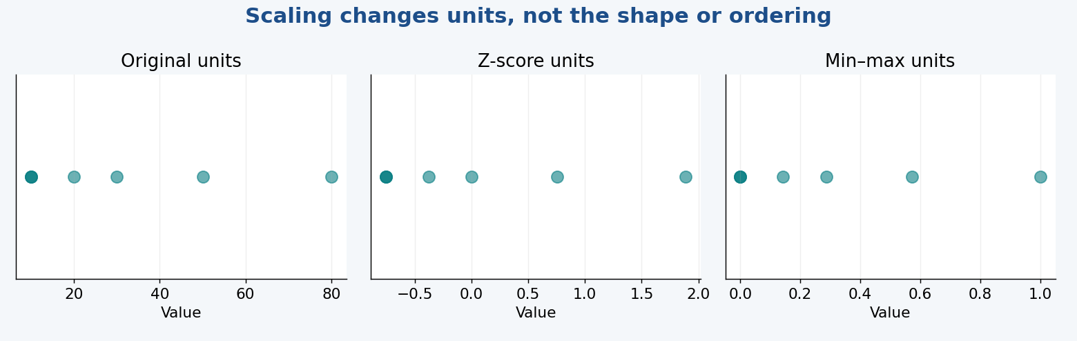
Scaling. Z-score = (value − mean)/SD; min–max = (value − minimum)/(maximum − minimum). These change units and preserve shape. Log changes shape but does not guarantee normality.
KNN. Neighbours depend on distance. Large numerical ranges can dominate, so a transformation can change neighbours and predictions.
Missingness. Inspect first; deletion, recoding and imputation serve different purposes. Filling a value does not make it measured. Choices depend on why data are missing.
mice. Chained-equation models create several plausible completed datasets. m = 5 creates five; complete(..., 5) extracts the fifth, not the best.
Networks. Layered weighted transformations can learn complex relationships, with more interpretability and overfitting concerns.
Risk and odds. Risk = events/all people; odds = events/non-events. RR compares risks, OR compares odds. The no-difference ratio is 1.
Communication. Report absolute risks with relative ratios. A doubling from 1 in 10,000 to 2 in 10,000 is different in practical scale from 20% to 40%.
What to be able to do
Be able to calculate a transformation, explain its consequences, choose missing-data handling and distinguish absolute risk, RR and OR. The example exams indicate question styles, not an exhaustive syllabus.
Distance-based algorithms treat numerical differences as meaningful. If one feature is height in metres and another is age in years, an age difference of 20 is numerically much larger than a height difference of 0.2. A nearest-neighbour model can therefore give age unintended influence just because of the units.
Scaling changes how features contribute to the model. It does not add observations or change the target labels.
Transformation
Formula
Main effect
Z-score standardization
z=(x-μ)/s
Express values relative to the mean, in standard-deviation units
Min–max scaling
(x-x_(min))/(x_(max)-x_(min))
Map the observed range to 0–1
Log transformation
log(x)
Compress large positive values more than small ones
Example: height 180 cm, mean 170 cm, SD 10 cm gives a z-score of 1. It is one SD above the mean. If the observed range is 150–200 cm, its min–max value is 0.6.
A clarification to the slides: z-scoring changes location and scale, not distribution shape. A skewed variable remains skewed. It does not make a variable normally distributed, and Gaussian data are not a prerequisite for using z-scores. Min–max scaling also preserves shape while changing scale. Log transformation changes shape and can reduce right-skewness, but does not guarantee normality or a 0–1 range.
A useful feature of logarithms is that ratios become differences: log(a)-log(b)=log(a/b). Ordinary logs require positive values.
2. The lecture’s nearest-neighbour example
The example predicts a category from height and age using k-nearest neighbours (KNN). KNN classifies an observation using nearby labelled training observations, so changing the distance calculation can change the prediction.
The slides report:
Preparation
Accuracy in the slide example
None
0.46
Z-score
0.54
Min–max
0.85
Log
0.85
The takeaway is scaling can strongly affect distance-based results. These scores do not establish that min–max or log transformation is always better. Note that the min–max code slide prints an accuracy of 0.769 (10 of 13 test students), while the summary slide lists 0.85; with such a small test set one prediction shifts accuracy by about 8 points. The slide code also rescales the test set with its own min/max rather than the training set's. Choose preparation for the features and model, then evaluate it.
For a training/test workflow, derive scaling parameters from training data and apply the same transformation to test data. Otherwise “the same value” can have a different meaning in the two sets. This is a practical clarification of the slide workflow.
3. Handling missing values
First inspect what is missing and what each field means. The lecture lists five possible actions:
Delete every incomplete row. Simple, but potentially discards a lot of information.
Delete rows missing a specific essential variable. More selective, but requires a reasoned choice.
Correct values that are wrong. In the recording the lecturer's example is a cell shown as NaN whose true value is simply 0 (e.g. no events), so you replace it with 0. The reverse also counts: a placeholder 0 that is really a missing measurement should become NA.
Fill with a meaningful category/value. Only when that value correctly represents the situation. “None” and “unknown” are not interchangeable.
Impute: estimate plausible values using the available information.
Imputation is an estimate, not recovery of the true missing value. Deletion and imputation can both distort conclusions if used without considering why values are missing.
4. What the mice example does
The slides show the mice package: multiple imputation by chained equations. Different incomplete variables are imputed using models appropriate for them.
Inspect the dataset and its missing values.
Ensure categorical variables are represented as factors.
Run mice() with suitable methods.
Inspect the generated imputations.
Use complete() to obtain a completed dataset.
The slide code uses m = 5 for five imputed datasets, maxit = 20 for twenty iterations, pmm for predictive mean matching and logreg for logistic-regression imputation of a binary variable. An empty method means that variable is not imputed.
complete(my_imp, 5) extracts the fifth completed dataset. The “5” identifies a dataset; it is not a quality score. Multiple datasets represent uncertainty in plausible replacements. Do not treat an imputed value as if it had been directly measured.
5. Neural networks versus simpler models
The slides compare a simple fitted function with a network learning more complex input–output relationships.
A neural network combines weighted inputs through layers of transformations. Training adjusts the weights to improve predictions. It can represent interactions and nonlinear patterns that a simple model may miss.
The trade-off is reduced interpretability and greater attention to overfitting, model complexity and data requirements. More complexity is useful only if it captures relationships that generalize. A simpler model is easier to explain and may work well when the features represent the problem clearly.
The deck names Bayes’ statistics in an outline, but does not develop a separate lesson on it. There is no extra Bayesian reading in this summary.
6. Probability, odds and ratios
Absolute risk is an event probability: events divided by everyone in the group. Odds compare events with non-events:
odds = (p)/(1-p)
If 20 of 100 people have an outcome, risk = 0.20, while odds = 20/80 = 0.25. These are different quantities.
Relative risk (RR) compares probabilities:
RR = frac(risk_(exposed))(risk_(unexposed))
Odds ratio (OR) compares odds:
OR = frac(odds_(exposed))(odds_(unexposed))
For either ratio, 1 means equal values between groups, greater than 1 indicates a higher value in the exposed group, and less than 1 a lower value.
Correction: the final slide’s “odds = 0: no difference” is misleading. A ratio of 1 means no difference; ordinary odds do not compare two groups. Likelihood is the probability/density of the observed data under a model as its parameters vary; it is not the same as R^2.
That means approximately 14.4 times the odds, not 14.4 times the probability. The corresponding risks are 31/37 ≈ 83.8% and 14/53 ≈ 26.4%; their RR is approximately 3.17. The difference illustrates why odds and risk must not be interchanged. Caveat: the slide shows two groups of 45 patients selected by disease status (with vs without heart disease), i.e. a case–control design. There the row “risks” (83.8% vs 26.4%) are not real population risks, so an RR cannot be estimated and the OR is the appropriate measure; the 3.17 only illustrates how far the two ratios can diverge.
Rare-event example: the slide table has 2 events plus 14,000 non-events in one group, versus 1 event plus 14,000 non-events in another. Correct denominators are therefore 14,002 and 14,001. Risks are approximately 0.0143% and 0.00714%, and RR is approximately 2.
The relative risk sounds large, but the absolute difference is only about 0.00714 percentage points, or roughly one additional event per 14,000 people in this example. The slide’s communication rule is to report absolute risks alongside relative comparisons.
Missing-data methods named in the sample
Mean replacement fills missing entries with a variable's average; it is simple but reduces variability and can distort relationships. Interpolation estimates a value between nearby known observations, usually in an ordered series such as time. It requires a sensible ordering and assumptions about the intervening pattern. Both are forms of estimating missing values; they do not create measured information.
the example exam asks which methods can be used in principle. Separate recognizing an available method from justifying it for the particular dataset.
Do the scaling arithmetic yourself
For an illustration with values 10, 20, 30, the mean is 20 and the sample SD is 10. Z-scores are −1, 0, +1. Min–max values are 0, 0.5, 1. Both preserve the ordering and distribution shape; they choose different numerical scales.
Subtracting only the mean centres the variable but leaves its variability unchanged. Dividing by SD makes the standard deviation one, allowing variables measured in very different units to be compared on a standardized scale. That does not guarantee equal scientific relevance or equal contribution to every algorithm.
With training minimum 10 and maximum 30, a future observation of 40 has min–max value 1.5. Values in the fitted training range map to 0–1; new values can lie outside it. If all training values are identical, the min–max denominator is zero and the feature needs special handling.
Missing-data decisions have consequences
Illustration: three observed training loads are 10, 20 and 30. Replacing a missing fourth value by 20 makes the completed data look less variable than many plausible alternatives. It creates an estimate, not another measured session.
Interpolation would be sensible only if the measurements are ordered and neighbouring values genuinely inform the gap. A missing athlete's injury category cannot be estimated merely by looking at the adjacent spreadsheet rows. Recoding an impossible zero as missing is different from inventing a replacement.
The mice workflow is a demonstration of fitting imputation models. Extracting one completed dataset does not capture all multiple-imputation uncertainty in a final scientific analysis; combined analyses use the multiple datasets. For predictive evaluation, fit preprocessing/imputation within training data or each training fold to keep validation information out of the fitting procedure.
Communicate changes in risk without exaggerating
Illustration: risks of 8% and 4% produce RR = 2, with an absolute difference of 4 percentage points. Their odds are 8/92 and 4/96, so OR ≈ 2.09. “Twice the odds” and “twice the probability” are different statements. The difference grows when events are common; OR and RR become more similar for rare events.
An OR/RR below 1 describes a lower relative value for the stated comparison. It does not automatically prove protection caused by an exposure. A ratio of 1 means equal odds/risks between compared groups, while an event probability of zero means no events under that probability.
Likelihood concerns how well different model parameters account for the observed data. It is not the future event probability, the event odds or R². The final slide's wording is loose; keep these definitions separate.
Try the interactive explanation
Open the scaling and risk page. Change a value to compare z-score and min–max units, and change event counts to see absolute risk, RR and OR diverge. These are teaching examples, not personal health recommendations.
From the recording
Points the lecturer made in the lecture recording on Canvas that are not (fully) on the slides. Times refer to the recording.
00:00 — Where scaling sits in the data science lifecycle: if you only change the scale of a feature (e.g. z-scoring, min–max, metres to centimetres) it counts as data preparation; if the transformation also changes the variability/shape of the distribution (e.g. a log transformation) it counts as feature engineering. (Slides p. 3 (lifecycle diagram showing both phases, no explanation))
02:06 — The standardization figure: a feature with mean ≈200 and SD ≈40 is z-scored, and the histogram keeps exactly the same shape; only the mean (now 0) and SD (now 1) change. So z-scoring does not create a normal distribution; the example was already normal. Exam note: the slide wording ('goal: acquire normal distribution') and the cheat sheet ('changes the original distribution if not Gaussian') suggest otherwise, but z-scoring is a linear shift-and-rescale that preserves shape. (Slides p. 5 (two histograms, not explained); p. 13 cheat sheet)
04:12 — The normalization figure: in the raw data Feature 1 has a much larger range than Feature 2, so in a distance-based model such as KNN the distance between two points is dominated by Feature 1 and Feature 2 is barely used. After normalization both have a similar range, so both contribute equally to distances. (Slides p. 5 (raw vs normalized scatter plots, not explained))
06:28 — Two practical steps in the R example. (1) Set a random seed before the random train/test split so the split is identical on every run; then differences between models (here the four scaling rounds) are not caused by different splits. (2) Plot height against age with a fixed 1:1 axis ratio to see what KNN 'sees': with height in metres the points form a flat line and distances are controlled by age; converting to centimetres already spreads them out, and ideally both features contribute equally (a round cloud). (not on slides (p. 7 code shows sample.split but no set.seed or plots))
08:35 — Emphasised: first split the data into training and test sets, then normalize/standardize, never the whole data set before splitting. The lecturer (and the slide code) scale the training and test sets separately; strictly, the standard practice is to compute the scaling parameters (mean/SD or min/max) on the training set and apply those same values to the test set. (Slides p. 8–10 (code applies scale()/normalize() to train and test separately; rule not stated))
10:40 — Accuracies as spoken: none 0.46, z-score 0.538, min–max 0.77, and log transformation 'even higher'. This matches the code output on p. 9 (0.769), not the 0.85 for min–max in the summary table, and ranks log as the best method in this example. Take-away the lecturer stresses: the choice of scaling alone has a large effect on accuracy of a distance-based model. (Slides p. 7–10 (code outputs) vs p. 12 (summary table))
12:46 — How a log transformation works (base 2): 1→0, 2→1, 4→2, 8→3, so equal ratios (fold changes) become equal steps and large values are pulled in towards the rest. That is why log is the method of choice for right-skewed features with some very high values/outliers. Min–max, by contrast, lets the extreme value set the scale ('puts a lot of value on outliers'), squeezing the other values together. ('Full changes' in the transcript is a mishearing of 'fold changes'.) (Slides p. 11 (log axis figure); right-skew advice not on slides (p. 13 cheat sheet omits it))
14:48 — Ranges after each method for height (raw about 1.5–1.96 m): z-scores about −1.7 to +1.8 (unbounded), min–max exactly 0 to 1, natural log about 0.41 to 0.67; a student of 1.70 m becomes ≈0.43–0.44 (min–max) and ≈0.53 (log). The lecturer calls log 'similar to min–max but with outliers counting less'. Correction: a log transformation does not map to a fixed 0–1 range; log(height) is 0.41–0.67 only because ln(1.5) ≈ 0.41, and log(age) on the same slide is 3.05–3.64. (Slides p. 12 (range() and summary() output, not interpreted))
20:55 — Meaning of option 3 'change values that are wrong (e.g. 0 instead of NaN)': the lecturer's example is a cell shown as NaN (not a number) whose true value is simply 0, so you replace it with 0. The reverse (a placeholder 0 that really is a missing measurement → NA) is also 'correcting a wrong value'. Before deleting rows, first check how much data is missing and how much you would lose. Imputation is the step to use only when the first four options are not possible. (Slides p. 15 (options listed; example not explained))
20:55 — Simplest imputation example: if the age of two students in the class is missing, impute it with the mean age of the whole group. Imputation = replacing a missing value with a best guess of what it could be. (not on slides (p. 15 gives the definition only))
25:01 — mice = Multivariate Imputation by Chained Equations (Whisper: 'change the equation'). In mice(), m is the number of imputations (multiple imputation) and method is set per column: "" for a complete column (nothing to impute), "pmm" (predictive mean matching) for numeric variables (bmi, chl) and "logreg" (logistic regression) for a binary variable (hyp, coded 1/2), which is why categorical variables must first be converted to factors. Advice: look up a new function's documentation (?mice) to understand its inputs. (Whisper's 'star wars' is a mishearing; the data set is nhanes.) (Slides p. 16 (code only; pmm/logreg not defined))
29:04 — Why impute several times: you can run your model on each of the m completed data sets; if the results differ a lot, the imputation is a big guess, and if they are close, it is fairly reliable. The lecturer said this is out of scope and that for the project it is fine to pick one completed set (he chose imputation 5 because its BMI values matched the observed mean of 26.56). Strictly, proper multiple imputation analyses all m sets and pools the results. (Slides p. 16 (steps 4–5 'choose the best matching imputation version'; rationale not on slides))
31:08 — Why classical models are preferred in this course over neural networks: in sport and health the aim is to find predictors and explain them to a practitioner, which needs an interpretable model; the hidden-layer nodes of a network are practically impossible to interpret. With a classical model you must handle relationships between inputs yourself (e.g. drop one of two strongly correlated features). Networks also need much larger data sets than the ~500-row sets used in the projects. Students are not expected to apply networks, only to have basic knowledge. (Slides p. 18 (pros/cons list without the reasons or examples))
35:11 — Neural network basics (IBM video): input layer, hidden layer(s), output layer; data pass forward layer by layer (feed-forward). Each node works like its own small linear regression: multiply inputs by weights, add a bias/subtract a threshold, and output 1 if the result is > 0. Surfing example: ŷ = 1×5 + 0×2 + 1×4 − 3 = 6 > 0 → output 1 (go surfing). Changing weights or threshold changes the decision. (Strictly, a node adds a non-linear activation, here a step function, so it is not just a linear regression.) (Slides p. 19 (video thumbnail only))
37:23 — How networks learn and which types exist (IBM video): they are trained with labelled data (supervised learning); a cost function measures the error and is minimised by gradient descent, which adjusts the weights and biases. Besides feed-forward networks there are convolutional neural networks (CNNs), suited to pattern/image recognition, and recurrent neural networks (RNNs), which have feedback loops and are used for time-series data to predict future events. (Slides p. 19 (video thumbnail only))
39:35 — Reading the odds ratio: OR = 1 means no difference in odds between exposed and unexposed; OR < 1 means lower odds of disease in the exposed group (exposure protective); OR > 1 means higher odds in the exposed group, so in the example smoking increases the odds of heart disease (OR ≈ 14.4). The spoken walkthrough garbles the cells (says '40' and calls smokers without disease 'unexposed'); correct: OR = (31/14)/(6/39) = (31×39)/(6×14) ≈ 14.4. (Slides p. 21 (formula and 14.4; interpretation only on p. 24))
43:50 — Absolute vs relative risk in the pill example: absolute risk on the pill ≈ 2/14,000 ≈ 0.00014; RR = 2, which the lecturer phrases as '200%' to show how alarming it sounds. Correction: RR = 2 means the risk is twice (200% of) the unexposed risk, i.e. a 100% increase, while the absolute increase is only about 1 extra case per 14,000. He also misspoke RR as 'unexposed to unexposed'; the slide's exposed/unexposed is correct. Hence: never report RR without the absolute risk. (Slides p. 22–23 (formulas and warning; percentage phrasing not on slides))
45:52 — The lecturer corrects slide p. 24 aloud: 'Odds = 0: no difference' should read 1: an odds ratio of 1 means no difference between groups, and odds/odds ratios range from 0 to infinity (probabilities 0–1). He says probability, odds and likelihood are terms students will very likely come across in the exam. He keeps 'R²' as an example of likelihood; strictly, likelihood is how probable the observed data are under a model's parameters, which is not R². (Slides p. 24 (says 'Odds = 0: No difference'; likelihood 'e.g. R2'))
Slide coverage map
Pages 1–3: scope/lifecycle; 4–13: scaling and the KNN example; 14–16: missingness and mice; 17–20: neural networks and outline transitions; 21–24: odds, absolute/relative risk and communication. “Bayes' statistics” appears in an outline but no separate Bayesian lesson is developed in this deck.
Worked through the deep dive?Tick it off. Come back to any section whenever you need it.
3Step 3 of 35–8 min
Practice questions
Exactly two original practice questions. These use the concept/application style of the 2024 and 2022–2023 example exams, with new scenarios and values. Try each before opening its answer. The official example exams are on Canvas; save them for a later, exam-style session.
Question 1 — Calculate and interpret scaling
For a training feature, mean = 50, SD = 10, minimum = 20 and maximum = 80. A value is 65. Calculate its z-score and min–max value. Does either transformation guarantee a normal distribution, and why might KNN predictions change?
Show answer and rationale
z = (65−50)/10 = 1.5; min–max = (65−20)/(80−20) = 0.75. Neither guarantees normality; both preserve distribution shape. Rationale: changing scale changes relative distances across features, potentially changing KNN’s neighbours. Use the same fitted training transformation on new observations.
How did your answer compare?
Question 2 — Compare risk and odds
In one exposure group, 12 of 100 people have an outcome; in the comparison group, 4 of 100 do. Calculate both absolute risks, RR, OR and the absolute risk difference. Give one clear sentence communicating the result.
Show answer and rationale
Risks: 12% and 4%. RR = 3. Odds: 12/88 and 4/96. OR = (12×96)/(88×4) ≈ 3.27. Absolute difference = 8 percentage points. One clear sentence: “The observed outcome occurred in 12% versus 4%, a threefold risk and an eight-percentage-point difference.” Rationale: OR is a ratio of odds, not probability; absolute figures prevent a relative comparison from hiding its practical scale. This table alone does not prove causation.