First read: about 4–6 minutes. Lecture 5: Regression.
Regression predicts a numerical target from predictors. This lecture links that task to feature construction, error metrics and regularization—the choices that help a model work beyond the examples it was trained on.
The ideas to keep
Blur the explanations and test yourself.
Learning types. Regression/classification use labelled targets; clustering finds groups without them; reinforcement learning uses rewards. Deep learning is a type of ML, while data science also includes acquisition and communication.
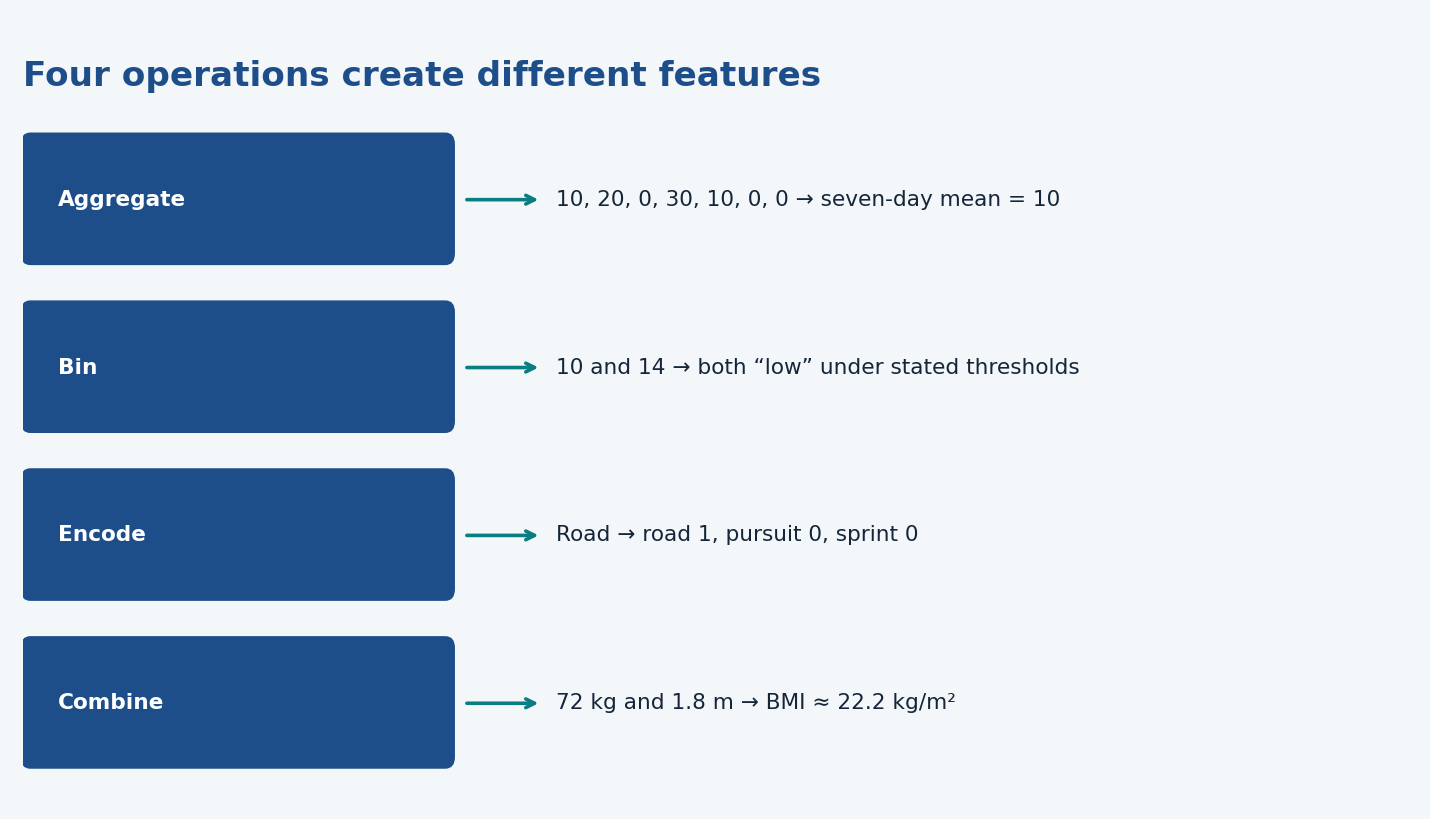
Useful features. Aggregation summarizes a variable over a window; binning creates categories; encoding represents category membership; combining variables creates a new quantity.
Error. MAE averages absolute residuals; MSE averages squared residuals and emphasizes large misses. Compare on observations that were not used to fit the model.
Overfitting. Zero training error can coexist with poor new-data predictions. A small or restricted sample makes estimates less reliable.
Regularization. Ridge adds a squared-coefficient penalty and shrinks coefficients. LASSO adds an absolute-coefficient penalty and can set some to zero. λ controls strength.
Validation and baseline. Tune using validation/CV and reserve final test data. Compare with a simple predictor-free benchmark before calling a model useful.
What to be able to do
Be able to identify target/predictors, explain feature operations, calculate MAE/MSE and justify ridge/LASSO and evaluation in a small-data scenario. The example exams indicate question styles, not an exhaustive syllabus.
Artificial intelligence (AI) is the broad idea of machines performing intelligent tasks. Machine learning (ML) is part of AI: models learn relationships from data. Deep learning is part of ML and uses neural networks with multiple layers. Data science overlaps with AI and ML, but also includes obtaining, preparing, exploring and communicating data.
Learning approach
What the model learns from
Example
Supervised regression
Inputs paired with numerical answers
Predict running time
Supervised classification
Inputs paired with category labels
Predict injury: yes/no
Unsupervised clustering
Inputs without target labels
Find groups of similar athletes
Reinforcement learning
Feedback or rewards from actions
Learn actions that help a robot navigate
A feature/predictor is an input column. The target is the answer you want to predict. Regression and classification both have targets; clustering does not have supplied “correct” group labels.
The lecture also introduces ensembles and neural networks. An ensemble combines models, such as several trees. A neural network learns a sequence of transformations from inputs to outputs. You mainly need to recognize these approaches here; ridge and LASSO are the detailed regression examples.
2. Feature engineering: make useful inputs
A model can only use the information represented in its features. Better features can make a simpler model sufficient: faster, easier to interpret and easier to maintain.
Operation
What you do
Example
Aggregate
Combine observations using a function and time window
Mean training load over seven days
Bin
Convert values into broader categories
Low, medium and high load
Encode categories
Represent categories as numerical indicator columns
A 0/1 column for each medal category
Combine variables
Create a feature from several existing variables
Body surface area from height and weight
One-hot encoding creates one indicator per category. Dummy encoding usually creates one fewer indicator, treating the omitted category as a reference. With an intercept in ordinary linear regression, including all category indicators creates a redundant representation: the indicators sum to 1, just like the intercept column. This is the dummy variable trap.
Example: with categories bronze/silver/gold, use bronze and silver indicators and let gold be the reference. A gold observation has 0 in both indicator columns.
3. Judge errors with the right metric
For observation i, the residual is y_i-ŷ_i: actual minus predicted value.
MAE: average absolute residual, (1)/(n)Σ |y_i-ŷ_i|. It reports the average size of the error in the target’s units.
MSE: average squared residual, (1)/(n)Σ (y_i-ŷ_i)^2. Squaring makes large errors count disproportionately. Its units are squared target units.
Both treat an overprediction and an equally large underprediction the same. MAE is less sensitive to extreme errors than MSE; it is not completely unaffected by them.
Worked example: residuals of 1, −1 and 4 give MAE = (1 + 1 + 4)/3 = 2, and MSE = (1 + 1 + 16)/3 = 6. One large miss dominates the squared-error score.
4. Training performance is not enough
In the holdout method, split the dataset into training and test data. Fit the model on training data, then predict the held-out observations and compare predictions with their actual targets.
Overfitting means learning a pattern too closely tied to the training observations, including noise. The lecture shows a steep line fitted perfectly through a tiny training sample, yet performing poorly on new points. Zero training error does not demonstrate good generalization.
5. Least squares, ridge and LASSO
Ordinary least squares chooses coefficients to minimize the sum of squared residuals. Regularization adds a cost for large coefficients, trading some training fit for a model that may generalize better.
Model
Objective in the lecture’s one-slope example
Effect
Least squares
Squared residuals
Best training fit under this criterion
Ridge
Squared residuals + λ × slope²
Shrinks coefficients toward zero
LASSO
Squared residuals + λ × abs(slope)
Can set coefficients exactly to zero
For multiple predictors, the penalty sums over their coefficients. λ (lambda) controls penalty strength: λ = 0 gives least squares; increasing λ strengthens shrinkage. Choose λ using cross-validation. Keep a final test set separate from tuning.
The slide calculation, λ = 1:
Steep least-squares line: 0 + 1.3² = 1.69.
Ridge candidate: 0.3² + 0.1² + 0.8² = 0.74.
LASSO objective for that candidate: 0.3² + 0.1² + |0.8| = 0.90.
The ridge candidate has a lower ridge objective despite having training residuals. This illustrates the effect of a penalty; it does not itself prove better test performance.
LASSO can remove unhelpful predictors by setting their coefficients to zero. Ridge usually keeps predictors while shrinking them. The lecture’s rule of thumb is LASSO when many predictors are unnecessary and ridge when most contribute. Treat that as a starting point, then compare validation performance.
Extra points made explicit by the example exam
Percentile versus minimum (the example exam): a minimum depends on one observation and may capture a sensor artefact. A less extreme percentile can reduce that dependence. Percentiles are not universally superior; the feature should represent the quantity you want.
Naive baseline (the example exam): compare predictions with a deliberately simple benchmark, such as always predicting the training-set mean. Beating it suggests added predictive value from the model/features. The sample describes a predictor-free baseline; “baseline” does not mean a perfect model.
Restricted range and poor fit (the example exam): a sample containing only very similar elite performers may have little variation in the target or a predictor. That makes a relationship harder to detect; low fit is not automatically proof that the predictor is irrelevant in a wider population. A small sample adds uncertainty.
Deep learning (the example exam): the sample emphasizes that deep models can learn intermediate features automatically, whereas conventional workflows often use manually engineered features. This is a typical contrast, not an absolute rule for every algorithm.
Walk through the four feature operations
Think of a feature as one piece of information placed in a column for a model. The four operations change how that information is represented.
Aggregate = summarize several observations into one value. Illustration: daily loads are 10, 20, 0, 30, 10, 0, 0. Their seven-day mean is 10. The variable is training load, the window is seven days, the function is mean. A sum would produce 70; a maximum would produce 30. These features answer different questions. A moving window is recalculated at each prediction date using only the relevant preceding observations.
Bin = put values into broader groups. If load 0–15 is called low, above 15 up to 30 medium, and above 30 high, loads 10 and 14 both become low. You gain a simple category but lose the difference between 10 and 14. Thresholds should be clear, with no overlap or gaps. Categorical binning also exists: Spain and Italy can be grouped as Europe, while Chile and Brazil can be grouped as South America.
Encode = represent a category in a form the model can use. A three-category discipline variable can become separate road/pursuit/sprint indicator columns. Each row has 1 in its category and 0 in the others. This represents membership; it does not say that sprint is three times road. In regression with an intercept, use a reference category to avoid redundant columns.
Athlete
Road indicator
Pursuit indicator
Sprint indicator
A, road
1
0
0
B, pursuit
0
1
0
C, sprint
0
0
1
Combine = calculate something from multiple variables. BMI combines mass with height: mass in kg / height in m squared. For mass 72 kg and height 1.8 m, BMI is 72/3.24 ≈ 22.2. The combining-variables slide illustrates this with BMI categories (and an image of airflow around a cyclist); in the recording the lecturer's example is BMI from height and weight. Body surface area is a further example of a height–mass feature, but it is not shown in the slides. The formula determines the meaning; simply adding measurements with different units usually does not.
Regression line: what intercept and slope say
In predicted size = 0.9 + 0.75 × weight, the intercept is the predicted size when weight is zero and the slope is a 0.75-unit increase in predicted size for a one-unit increase in weight. The intercept may lie outside the meaningful data range, so do not necessarily give it a literal biological interpretation.
Least squares minimizes vertical squared residuals in the target. That is not the same geometric operation as PCA, which seeks directions of greatest variance. A very steep line fitted through only two training points can be unstable: small differences in the sample can change its predictions substantially.
Regularization deliberately accepts more training error if the penalized objective improves. In the lecture's small example, the training data—not the test data—are what the steep line overfits. One slide reverses that wording. Keep the final test set unseen during model and λ selection.
Broader methods introduced in the first half
Reinforcement learning learns actions using reward feedback, such as navigation or games. It is not the same task as predicting a labelled race time.
An ensemble combines models. Random forests combine varied trees; boosting builds successive models that improve the ensemble. These approaches are not inherently perfect or automatically better for every dataset.
A neural network learns weighted transformations. Deep learning uses multiple layers to learn intermediate representations, which can be useful for images, speech and other complex inputs. Humans still choose data, targets, architecture and evaluation. The slide's “without human intervention” description concerns learning parameters from data, not the entire scientific workflow.
AI, ML and deep learning have a nested relationship, while data science overlaps with them and also includes work that uses no AI. A neural network is not required for a useful data science result.
Try the interactive explanation
Open the regression and shrinkage page. Move the line and inspect residuals, MAE/MSE and penalty strength. All points are invented teaching data. The fixed-data demonstration illustrates the objective; it cannot prove a model will generalize better.
From the recording
Points the lecturer made in the lecture recording on Canvas that are not (fully) on the slides. Times refer to the recording.
00:45 — Checking an imputation (Lecture 4 topic, from a student question): there is no single rule for using the same imputation method for every variable or a different one per variable. A different method per variable makes sense when the variables have different distributions (e.g. one normal, one not). The only rigorous check is to remove values you actually know, impute or predict them, and compare with the true values. The practical advice was to impute, plot the data and accept the imputation if the imputed points fall within the expected distribution rather than showing up as outliers. (not on slides)
27:30 — A regression function need not be linear. In long jump, distance increases with approach speed only up to an optimum, after which ground contact is too short to take off well, so a straight line fits only part of the data and a quadratic (optimum) or polynomial function fits better. The trade-off is that higher-order functions are harder to interpret ('more is better' holds for only part of the curve), and predictions can be badly wrong for new data that come from outside the training distribution. (Slides p. 12 (linear vs polynomial fit to traffic-jam data, no explanation))
33:15 — Supervised algorithms usually test hypotheses, whereas unsupervised algorithms usually generate them: you often end up with more questions than answers. Example: cluster only the 100-m times of sprinters and long jumpers into two clusters without giving labels. If each cluster mixes both groups, the discipline label does not seem to define sprint ability. That suggests the hypothesis that other factors do, and the same data with labels would instead be a supervised classification. (not on slides (p. 13 only defines clustering as dividing objects by unknown features))
34:00 — Know the vocabulary of reinforcement learning, which the lecturer said you 'should know': correct decisions are rewarded and wrong decisions are penalised, so the algorithm improves over many training cycles (Pac-Man example: thousands of cycles before it won all its games). She said it can be supervised or unsupervised. The slides draw it as a separate third branch next to supervised and unsupervised learning. (Slides p. 14–15 (robot in maze, list of uses, video), p. 8–9 (separate branch). The reward/penalty mechanism is not written out.)
37:20 — Ensemble (boosting) idea: train a first model (e.g. a decision tree that is only about 50% correct), then train the next model on the errors of the previous one, and repeat, so each model learns from its predecessor's mistakes. Different algorithm types can also be stacked (e.g. regression followed by classification). Correction: the lecturer said you repeat 'until you have a perfect prediction'. In reality boosting improves the fit but does not guarantee a perfect prediction, and it can overfit. (Slides p. 17 ('stupid trees learning to correct errors of each other'), p. 16)
41:20 — A neuron computes a weighted sum of its inputs. Each weight expresses how important that input is (for 'apple', a round shape matters more than 'grows on a tree'). If the sum passes a threshold, the neuron outputs 'yes'. When a prediction is wrong, the weights are adjusted, and learning means adjusting the weights. Slide example: 10×0.5 + 7×1.0 + 3×0.1 = 12.3 > 10, so the output is 1 (yes). (Slides p. 19 (neuron sum diagram and MLP, no explanation of weights))
46:00 — Deep learning means neural networks with more than one layer. Its advantage is automatic feature extraction: you input everything and the network decides which inputs matter, whereas in 'shallow' (classical) ML you choose and engineer the features yourself. Its cost: you lose control and context. Domain knowledge is not contained in the numbers, so the network may drop a meaningful predictor, e.g. physical activity for resting heart rate if the correlation is weak. It is also a black box: the weights are spread over many connections, so it is very hard to trace which information drove a prediction, while movement scientists want to know what makes someone, say, a good sprinter. For simple data sets, shallow ML gives the same result, so 'keep it simple'. (Slides p. 20–21 show the two workflows (feature extraction then classification vs combined). The trade-off is not on slides.)
54:30 — Reading the performance-versus-data curve: with little data, both approaches perform similarly. Shallow ML plateaus because it has a limited number of possible connections (one layer), whereas deep learning keeps improving because it can form many more connections as data grow. Human movement science data sets are usually small, so pick the simpler method. Large data sets from markerless motion capture and wearables now make deep learning feasible, e.g. predicting ground reaction forces from one IMU on the shank. (Slides p. 23 (curve only, no explanation))
68:30 — Selecting predictors by correlating every candidate variable with the target, or by putting everything into one multiple regression, shows that you have no hypotheses, and it misses combinations and interactions of variables. Choose features by reasoning about plausible relationships. Fewer good features give a simpler model (5 good features versus 50), and the choice of features determines the model's fit. (Slides p. 30 only says better features mean simpler models and better results. The critique is not on slides.)
71:00 — Aggregation examples for time-series data (e.g. joint angles over time to classify gait): cut the signal into windows (e.g. each cycle from valley to peak to valley), take a summary such as the window mean, or fit a function (e.g. a 2nd–3rd order polynomial) and use its parameters instead of thousands of raw points. Aggregating means simplifying the data while still representing the original. (Slides p. 31 (lists only 'Window' and 'Function'))
75:50 — Terminology warning: the lecturer said the terms the wrong way round. She said one-hot encoding 'uses fewer columns than you have categories' (male and female columns, with 'neither' coded 0, 0). The slides and standard usage say the opposite: one-hot = one column per category (k columns), dummy encoding = k − 1 columns, with the reference category coded as all zeros. Go by the slides. (Slides p. 34 (one-hot: d1–d3 for Red/Green/Blue), p. 35 (dummy encoding: d1–d2, Blue = 0, 0; 'dummy variable trap'))
77:00 — Do not code a nominal category as a single numeric column (Italy = 1 … United States = 100). The algorithm reads the numbers as ordered quantities, so a 'bigger' code can create a spurious relationship (e.g. with salary). Use indicator columns (dummy/one-hot) so that no category gets extra weight just because of its number. (not on slides)
82:50 — A downside of both MAE and MSE: because the sign is removed, they cannot show whether the model systematically under- or over-predicts. If the direction of the error matters, inspect the signed residuals as well. She called MSE the more commonly used metric. (Slides p. 41–42 state 'deviations in either direction are treated the same way' but not this consequence)
83:50 — Fitting a model to the whole data set and reporting a high r or R² (e.g. 0.9) is 'only half the story': it shows that the model fits these data and that the variables are related, not how well it predicts new cases. Prediction must be evaluated on data that were not used to fit the model. (not on slides (p. 39–40 only ask for generalizable results))
85:30 — Cross-validation was strongly emphasised ('I will hammer it into you'). The lecturer's description was muddled: she spoke of training on partition 1, then 2 … 10, comparing r and keeping the 'best partition'. The correct description of k-fold CV: split the training data into k folds (e.g. 10). In each round, train on k − 1 folds and evaluate on the left-out fold, so that every fold is held out once, then average the error. CV is used to tune and compare models (e.g. choose λ) and to see how much results depend on the partition, which can expose outliers. You do not select a single 'best' partition. (Slides p. 43 (CV = re-sampling procedure for assessing generalization), p. 45. The k-fold mechanics are not on slides.)
87:10 — Holdout rules: split off the test set (typically about 20%, with about 80% for training, which is not a hard rule) before modelling, and 'really never touch it' until all modelling is done, otherwise 'it's cheating'. At the end, apply the trained equation to the test predictors and compare the predictions with the actual values. That agreement is the model's performance. Ideally the test data come from a different source or lab (external validation). (Slides p. 44–45 (holdout definition and workflow). The 80/20 split, 'cheating' and external lab are not on slides.)
90:40 — Data leakage: when a person has several rows (longitudinal or repeated-measures data), split by person. Each athlete goes entirely into training or entirely into test, never both, and CV folds should also be split by athlete. Otherwise the athlete's characteristics leak into training and the results look too good. With one row per person, a random 80/20 split of rows is fine. Remove true duplicate rows (keep one), otherwise that case gets extra weight. (not on slides (the term 'data leakage' does not appear))
98:30 — The lecturer correctly says that the steep two-point line overfits the TRAINING data: a perfect fit on training data and a bad fit on test data. This confirms that the slide's wording 'overfit to the testing data' is a slip. Least squares has no way to tell the model its fit is 'too good', which is the motivation for ridge. (At 99:30 she also slipped and said 'fit the testing data not perfectly', meaning the training data.) (Slides p. 49 (says 'New line is overfit to the testing data'))
102:30 — Correction to the spoken ridge calculation: she said the residuals were 0.3 and 0.2 and to 'sum them up and square them'. The slide uses 0.3 and 0.1, squaring each and then summing: 0.3² + 0.1² + 1 × 0.8² = 0.09 + 0.01 + 0.64 = 0.74, versus 0 + 1 × 1.3² = 1.69 for the least-squares line. Use the slide numbers. (Slides p. 52)
104:20 — Why ridge prefers a flatter slope: with a steep slope, tiny predictor differences produce large prediction differences (100 g of weight 'predicting' 1 m of height is absurd). A flatter slope makes predictions less sensitive and tolerates more variability, which helps on test data whose spread differs from the training data. Correction: she said a 45° slope corresponds to 'an R-value of one'. The slope and the correlation r are different things: r = 1 means all points lie on a line, whatever the slope. (Slides p. 53–56 (sensitivity explanation). The r misstatement is verbal only.)
109:50 — LASSO versus ridge: she read the rise from 0.74 (ridge cost) to 0.9 (LASSO cost) for the same line as 'this variable gets less weight'. Strictly, costs from different objectives cannot be compared. The real reason is the penalty shape: for slopes below 1, |slope| is larger than slope², and the absolute penalty keeps pulling just as hard near zero, so LASSO can set a slope exactly to 0 (removing the variable). Ridge's pull fades as the slope approaches 0, so it shrinks the slope but never reaches 0. In the summary figure, as λ increases, the ridge minimum moves towards 0 but stays above it, while the LASSO minimum lands exactly on 0. (Slides p. 58 (LASSO 0.9 calculation), p. 59 (cost curves for λ = 0–400 and λ = 0–40))
Slide coverage map
Pages 1–24 introduce AI, ML, learning types, ensembles and deep learning; 25–36 develop targets, predictors and features; 37–47 cover error metrics, holdout and workflow; 48–60 work through least squares, ridge, LASSO and λ. The diagrams and arithmetic above cover the conceptual content; the original slides retain the full illustrations.
Worked through the deep dive?Tick it off. Come back to any section whenever you need it.
3Step 3 of 35–8 min
Practice questions
Exactly two original practice questions. These use the concept/application style of the 2024 and 2022–2023 example exams, with new scenarios and values. Try each before opening its answer. The official example exams are on Canvas; save them for a later, exam-style session.
Question 1 — Choose a model and evaluation plan
You have 48 athletes, 16 candidate measurements and a numerical target: recovery time in days. Several measurements may add little predictive information. Choose a model family, explain why LASSO might be worth comparing with least squares, and describe how you would evaluate it without tuning on the final test results.
Show answer and rationale
Supervised regression, because the target is numerical and supplied for training. LASSO penalizes absolute coefficients and can remove unnecessary predictors by setting them to zero, which can help control overfitting in a small dataset. Tune λ through cross-validation inside training data, fit preprocessing within those folds, and reserve a final test set where feasible. Compare with a simple mean-prediction baseline. Rationale: no penalty guarantees better predictions; use unseen-data evaluation rather than selecting the best training fit.
How did your answer compare?
Question 2 — Calculate and interpret errors
Actual times are 40, 45 and 50 minutes; predictions are 42, 44 and 46. Calculate MAE and MSE, including units. Then explain how “average distance over the preceding 14 days” differs from binning daily distance into low/medium/high.
Show answer and rationale
Residuals: −2, +1, +4 minutes. MAE = 7/3 ≈ 2.33 minutes. MSE = 21/3 = 7 minutes². Squaring makes the four-minute miss count much more. Aggregation summarizes several distances using a mean and a time window; binning converts individual values to broader category labels, losing within-category distinctions. Rationale: both are feature operations but change different aspects of the data.