First read: about 4–6 minutes. Lecture 3: Data in sport and health.
This lecture asks how to find and organize sport/health data. It uses a cyclist study and speed-skating results to show that useful acquisition starts with a question, then connects files, APIs and analytical storage.
The ideas to keep
Blur the explanations and test yourself.
Data sources. Performance, tests, videos, questionnaires, sensors and diagnoses offer different information and quality limitations.
Cycling case. Wingate and a 15 km time trial measure sprint/endurance. Multilevel physiology illustrates why selecting meaningful variables requires domain knowledge. Association is not an intervention effect.
Acquisition. Scraping extracts information from web pages; an API is a defined software interface. JSON/XML can carry the responses. Neither method guarantees accurate data.
Storage. A database organizes records; a warehouse integrates sources for analysis; a mart focuses on one area; a lake retains original structured/unstructured data for later use.
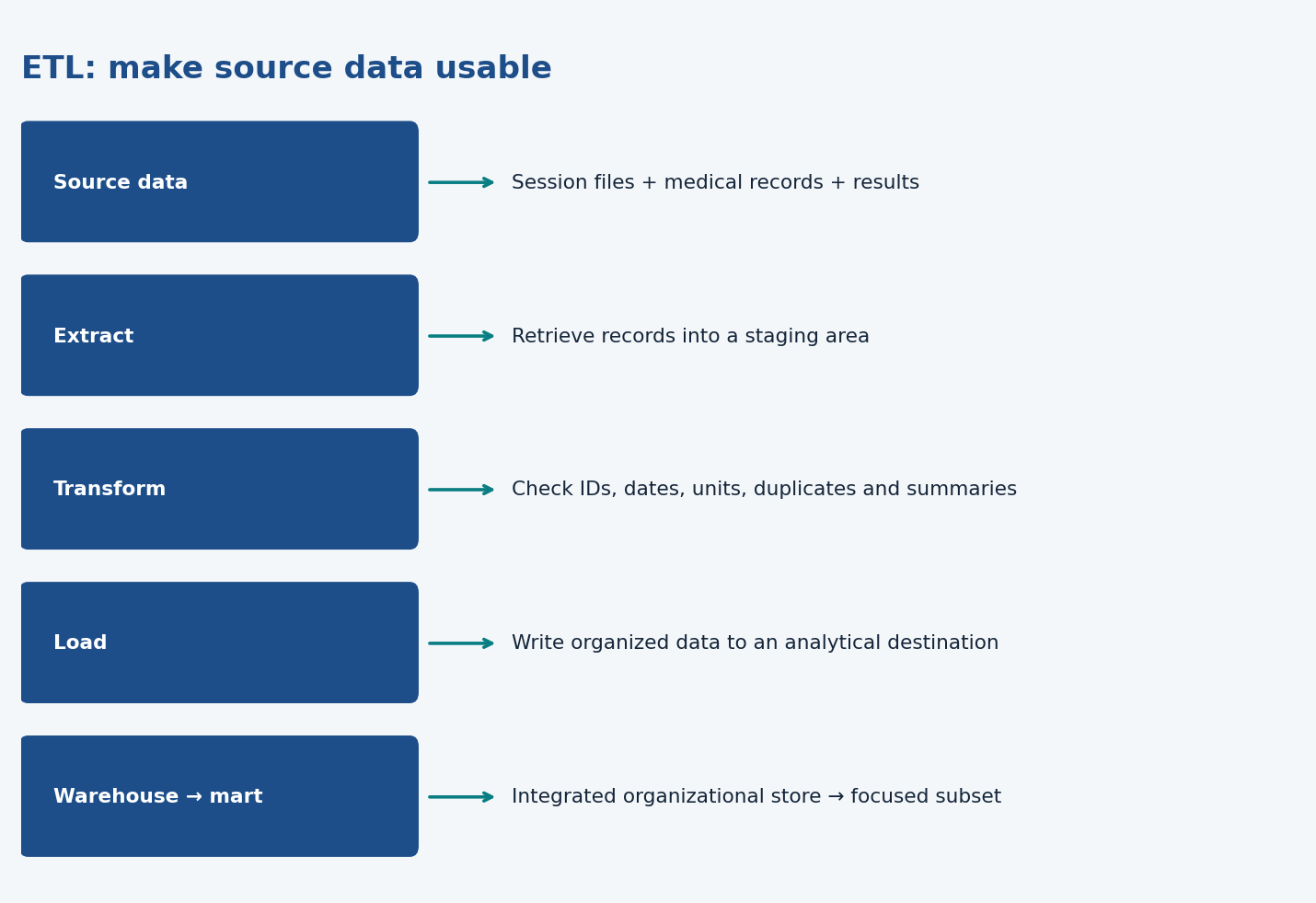
ETL. Extract source data, transform formats/units/structure and check them, then load an analytical destination.
Skating example. Compare seasonal performance with the world record on the race date and show specialization and track context. A larger raw time ratio means slower relative performance.
Range matters. An elite sample with little variability can hide a relationship. No detected association in that sample does not prove irrelevance everywhere.
What to be able to do
Be able to choose a source/store, explain ETL and API versus scraping, and connect the study question to its measurements. The example exams indicate question styles, not an exhaustive syllabus.
Got the big picture?Mark the overview done to fill this lecture's ring.
2Step 2 of 312–18 min
Detailed notes
Source:full presentation. Canvas lecture page checked 11 October 2026, 11:40 CEST. Existing lecture transcript used to clarify demonstrations; its older administrative dates are excluded. Examples labelled “illustration” are invented to explain the slide concepts.
Acquisition means obtaining information that can answer a question. Ask: what do I need, where is it, how can I obtain it, and how should it be stored and accessed? Do this before collecting everything you can find.
The lecture connects three topics: examples of sport/health measurements, ways of acquiring and storing them, and extract–transform–load (ETL). Acquisition and preparation overlap: an imported table often needs transforming before you can use it.
Categories and value of sport/health data
Category in the slides
Example
What to think about
Performance
Race results, sprint power
Event, units and testing conditions
Physical tests
Strength, oxygen uptake
Protocol and measurement reliability
Video/imaging
Match video, ultrasound, radiology
Features must be extracted and validated
Questionnaires/training schemes
Symptoms or planned sessions
Wording, self-report and planned versus completed training
Sensor data
Heart rate, movement
Noise, wear time, timestamps
Diagnosis
Clinical outcomes
Definition and completeness
Radiology illustrates potential benefits from recognizing patterns and screening abnormalities faster. Those potential benefits still need evaluation; using AI does not guarantee fewer errors.
The insurance activity example illustrates commercial value from tracking goals, activity and personal health information. Ask whose interests a use serves and what consent/privacy conditions apply.
Fitbit resting-heart-rate data illustrate scale and subgroup comparisons: age, sex, BMI and physical activity may all relate to resting heart rate. The slides ask students to sketch expected relationships between activity minutes and resting heart rate for men and women. A reasonable hypothesis is lower resting heart rate with greater activity, with diminishing changes. Slide p. 11 asks for expected cut-off numbers and slide p. 12 shows the result: resting heart rate falls steeply, then levels off from roughly 200–250 active minutes per week, with women higher than men at every activity level (consistent with the 150–300 min/week activity guideline). Resting heart rate is influenced by many other factors, including medication, hydration, stress and body size.
Detailed case: combining sprint and endurance
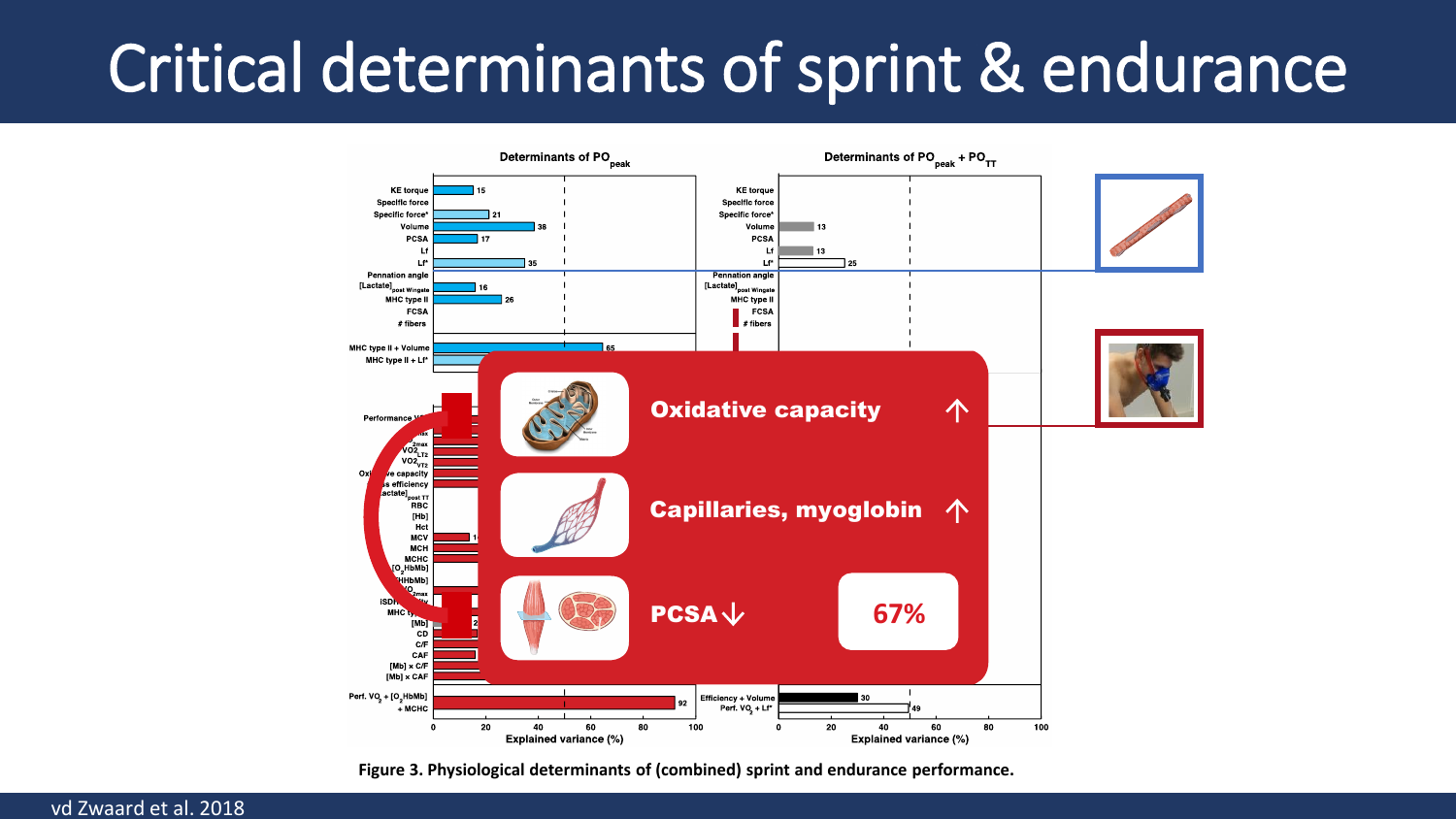
The van der Zwaard example asks which physiological characteristics relate to achieving both high sprint and endurance performance. Sprint performance benefits from the capacity to produce high force/power; endurance requires sustained energy production and oxygen supply. Large muscle fibres can create a challenge for oxygen delivery, so excelling in both is not simply a matter of maximizing every variable.
The slides describe 28 cyclists, including sprint, team-pursuit and road athletes, competing up to Olympic level. Performance was assessed with a Wingate test for sprint and a 15 km time trial for endurance. Candidate determinants were measured at several biological levels:
Level
Measures shown
Whole-body exercise
VO₂max, oxygen uptake during performance, lactate and ventilatory thresholds, gross efficiency
Blood/oxygen transport
Lactate, oxygenation, haemoglobin, haematocrit, red cells and related blood indices
Muscle structure/function
Ultrasound-derived volume, fascicle length, pennation angle, physiological cross-sectional area (PCSA), torque and specific force
Muscle fibres
Fibre type, fibre cross-sectional area (FCSA), fibre number, oxidative capacity, myoglobin and capillaries
FCSA is the area of an individual fibre. PCSA describes a muscle's effective cross-sectional area related to force production; these are not the same measurement. Gross efficiency relates useful mechanical work to energy expenditure. Capillaries deliver blood, and myoglobin supports oxygen availability within muscle.
The visual argument is that sprint and endurance performance trade off, but examining combinations of determinants can reveal profiles compatible with better combined performance. The slides emphasize long muscle fibres, capillaries/myoglobin and oxidative capacity in this explanation. Mind the direction for PCSA: a small PCSA (less hypertrophy) helps. High oxidative capacity, capillaries × myoglobin and a small PCSA together explained 67% of the variance in performance VO2 (R² = 0.67), a key determinant of combined sprint–endurance performance. Their result diagrams include study-specific percentages; they describe fitted relationships in this sample, not guaranteed gains from a training intervention.
The transcript discusses Deming regression as a way to study a relationship when both measurements have error, and warns about restricted range. If all participants are very similar in a predictor, it becomes hard to identify its relationship with performance. This can occur in an elite sample even when the variable matters in a broader population. A small sample also makes estimates uncertain. The lecturer explicitly treats the study as an example of using data and modelling; understanding the logic is more useful than memorizing every coefficient.
Do not jump from association to “this training causes improved performance.” The measurements can suggest hypotheses and potential targets for training; establishing intervention effects needs appropriate evidence.
Files and databases
A spreadsheet or CSV can be sufficient for a small table. A database becomes useful when data grow, several tables relate to each other, or you need repeated efficient queries.
The slides contrast legacy .xls limits (65,536 rows, 256 columns) with .xlsx (1,048,576 rows, 16,384 columns). CSV has no comparable built-in worksheet dimensions, but “unlimited” in the slide does not mean infinite practical storage: memory, software and file size still limit handling.
A relational database stores related tables. For example, one table stores athlete details, another sessions, and another measurements. An athlete ID connects records without repeating all personal details in every row. Indexing helps retrieve relevant records. SQL is a language commonly used to query relational databases; NoSQL refers to other database approaches.
Web scraping and APIs
Web scraping retrieves and parses website content to extract information. An application programming interface (API) provides a defined interface through which software requests data or operations. An API is not the database itself; it governs access to functions or information exposed by a service.
Illustration: a web page displays race results. Scraping reads the page's layout. An API may instead let a program request an athlete's results directly in a structured response. Changes to page layout can break a scraper, whereas API users rely on the documented request/response structure, which can also change.
Requests typically use HTTP. The slides show JSON and XML as formats for representing exchanged information. You need to know their role, not memorize their full syntax. Providers include companies, governments, leagues, publishers and individuals. Availability and permissions are separate questions.
Speed-skating API case
The example obtains world-record progressions, seasonal bests and athlete information from a results service. It asks how to visualize talent development across seasons.
The comparison uses an athlete's seasonal-best time relative to the world record on the race day, rather than today's record. A ratio seasonal best / world record = 1.2 means the athlete took 120% of the record time: 20% longer. A ratio of 1 means equal time.
Important visual distinction: for this raw time ratio, smaller is better. The slides say “bigger is better” for the graphic's performance presentation, which must use an appropriate plotting direction/transformation. Do not interpret a bigger raw time ratio as faster skating.
The graphic's direction/shape shows specialization across sprint, middle and long distances; size conveys level; track symbols distinguish indoor/open and highland/lowland conditions; a circle marks a record. Animation shows seasonal development. The full deck preserves the figure; a single number should not replace its multidimensional information.
Storage concepts, explained as a useful map
Store
Role
Sports illustration
Database
Organized data for storage and retrieval; many possible designs
Athlete and session records linked by IDs
Data warehouse
Integrates data from several sources for organizational reporting/analysis
Club-wide performance, medical and administrative information
Data mart
Focused subset for a department or purpose
Coaching department's training summaries
Data lake
Retains structured and unstructured data in original formats for later use
Raw sensor files, video and tables
A warehouse can contain detailed, summarized and metadata records. The deck mentions large warehouse sizes and denormalization for read/query performance; these describe common designs, not universal minimum-size definitions. A mart's focus is narrower than a warehouse's. A lake's flexibility shifts more of the interpretation/processing work to later use.
ETL: extract, transform, load
Extract: retrieve records from source systems. A full extraction retrieves everything; a partial/incremental extraction retrieves new or changed records. A staging area temporarily holds incoming data.
Transform: make the data usable for the destination. The lecture lists cleaning, format revision, threshold validation, restructuring, deduplication, filtering, merging, splitting, derivation, summaries, integration and aggregation. These are different operations, not one magic “clean” button.
Load: write the transformed records to the destination, such as a data warehouse, for analysis or business-intelligence tools. Check the staging data first.
Illustration: export separate training files → standardize athlete IDs, timestamps and units, remove accidental duplicates, calculate daily totals → load the consistent daily table into the club's analytical store. A lake might retain the original exports alongside that processed table.
The lecture briefly names Sport Data Valley as a sport-data platform context. This does not replace the principles: define your question, choose appropriate sources, organize data and check how transformations affect meaning.
From the recording
Points the lecturer made in the lecture recording on Canvas that are not (fully) on the slides. Times refer to the recording.
05:04 — Structured vs unstructured by category: performance and sensor data are mostly structured; video/imaging is mostly unstructured but becomes structured once features are extracted (e.g. markerless motion-capture landmarks in a table); physical tests, questionnaires and diagnosis can be either (Borg score, closed answers, injury yes/no = structured; open interview answers or a verbal clinical judgement = unstructured). (Slides p. 6 (categories only))
12:42 — Team tracking data (GPS, heart rate, acceleration for every player) are high-dimensional; summarising them into simple team metrics such as surface area covered and team length is dimensionality (complexity) reduction, a core theme. The aim is to let a model rather than the researcher choose the variables, which is more objective. (Slides p. 7 (image only))
14:44 — AI in radiology detects abnormalities from grey-scale patterns without context and is more consistent than human raters (whose reading depends on training lab and daily state), but context still matters, so a clinician should interpret after machine pre-screening. (Slides p. 8 (benefits only))
20:06 — The ASR activity-discount scheme did not make inactive people active: it mainly rewarded people who were already active, and losing the discount acted as a punishment. Individual incentives do not solve a systemic problem. (Slides p. 9 (scheme only, no outcome))
23:29 — Fitbit results: women have a higher resting heart rate than men (one explanation: smaller heart); resting HR vs BMI is U-shaped with an optimum in the normal BMI range (very low BMI also raises resting HR). (Slides p. 10 (graph only))
34:33 — Resting heart rate falls with weekly active minutes along a levelling-off (hyperbolic) curve, with women offset above men; the plateau starts around 200–250 min/week, consistent with the 150–300 min/week activity guideline. (Slides p. 11–12 (question and graph only))
37:48 — Wider error bars at the extremes of a plot (e.g. very low or very high BMI) mainly reflect few participants there, so interpret those points cautiously. Strictly, the standard error/CI depends on n, not the SD (the lecturer said SD). (Slides p. 10 (graph only))
46:16 — A correlation is not a percentage of explained variance: r = −0.66 between sprint and endurance means r² ≈ 0.44, i.e. about 44% shared variance (the lecturer said '36–40%', which is a slip). (Slides p. 23 (r only); rule on Lecture 4 slides p. 53)
48:31 — Ordinary least squares minimises vertical (or horizontal) distances to the line, treating one variable as error-free; van der Zwaard et al. used Deming regression, which minimises perpendicular distances and accounts for error in both variables; the perpendicular residuals quantify combined sprint + endurance performance. (Slides p. 24–26 (perpendiculars drawn, method not named))
54:16 — High oxidative capacity, more capillaries × myoglobin and a SMALL PCSA together explained 67% of the variance in performance VO2 (R² = 0.67), a key determinant of combined sprint–endurance performance. The lecturer phrases it as 'explains combined performance by 67%'; strictly the 67% is for performance VO2. A large muscle cross-section (hypertrophy) works against oxygen use. He does not expect you to know the coefficients — know the method (multiple regression on combined determinants). (Slides p. 28)
63:58 — Restricted range: if a predictor barely varies in the sample (pennation angle in elite cyclists) or the outcome barely varies (top-10 marathon times seconds apart vs varying VO2max), no relationship can be detected even if one exists. Always check the variability of every variable before regression. (not on slides)
66:46 — Before collecting, decide which data you actually need to answer the question: this concerns efficiency and storage, and is also an ethical issue (do not burden participants with unnecessary measurements). (Slides p. 33 (questions only))
81:27 — In the speed-skating radar chart, 1.0 (= world record) lies on the outer rim and slower ratios (e.g. 1.2) lie toward the centre, so 'bigger is better' refers to a larger filled area, not a larger ratio. (Slides p. 49 and 51)
83:42 — Public or scraped data have unknown quality: screen for outliers and missing values, compare with the expected measurement error for that data type, and cross-check sources; reporting standards (system used, capture frequency, cleaning already done) are still being developed. (not on slides)
98:11 — A data lake is low effort to store into but high effort to reuse; organising data into data marts makes it reusable by others. (Slides p. 64–65 (definition only))
99:10 — For every assigned paper, know which statistical model was used and why: read the methods and results sections. (not on slides)
Slide coverage map
Pages 1–4 introduce acquisition; 5–14 show data categories and value; 15–32 develop the cycling study; 33–51 cover storage, scraping, APIs and skating; 52–65 cover warehouses, ETL, marts and lakes. Repeated result figures and visual-only examples remain available in the local PDF.
Worked through the deep dive?Tick it off. Come back to any section whenever you need it.
3Step 3 of 35–8 min
Practice questions
Exactly two original practice questions. These use the concept/application style of the 2024 and 2022–2023 example exams, with new scenarios and values. Try each before opening its answer. The official example exams are on Canvas; save them for a later, exam-style session.
Question 1 — Choose the store
A federation wants to keep original match videos, raw sensor files and tabular results for analyses that have not yet been planned. Which store best fits that description?
A. A narrowly focused data mart.
B. A data lake.
C. A summary chart.
D. A single filtered data frame.
Show answer and rationale
B. A data lake. It retains original structured and unstructured formats for later analysis. A mart is focused on a particular purpose; a chart or filtered table is already a specific derived representation.
How did your answer compare?
Question 2 — Acquisition and ETL
A website publishes yearly athlete results and also offers an interface that returns results as JSON. Explain API versus scraping, then give one example action for each ETL step if you combine results across years.
Show answer and rationale
API: request results through the service’s defined software interface. Scraping: retrieve/parse displayed web-page content. Extract: obtain yearly records. Transform: standardize athlete IDs, units and year fields, investigate duplicates. Load: store the consistent results in an analytical database/warehouse. Rationale: obtaining data and organizing it for use are related but distinct operations; an API does not remove the need for quality checks.