First read: about 4–6 minutes. Lecture 2: Programming in R.
R is a language for telling a computer what to do with data. This lecture starts with values and containers, then teaches selecting data, using functions, and repeating or branching instructions.
The ideas to keep
Blur the explanations and test yourself.
Objects and assignment. height <- c(168, 182) stores a vector. mean(height) applies a function. Names are case-sensitive and indexing starts at 1.
Types. Numbers, text and logical values behave differently. NA is unknown/missing; NULL is absence of an object/value.
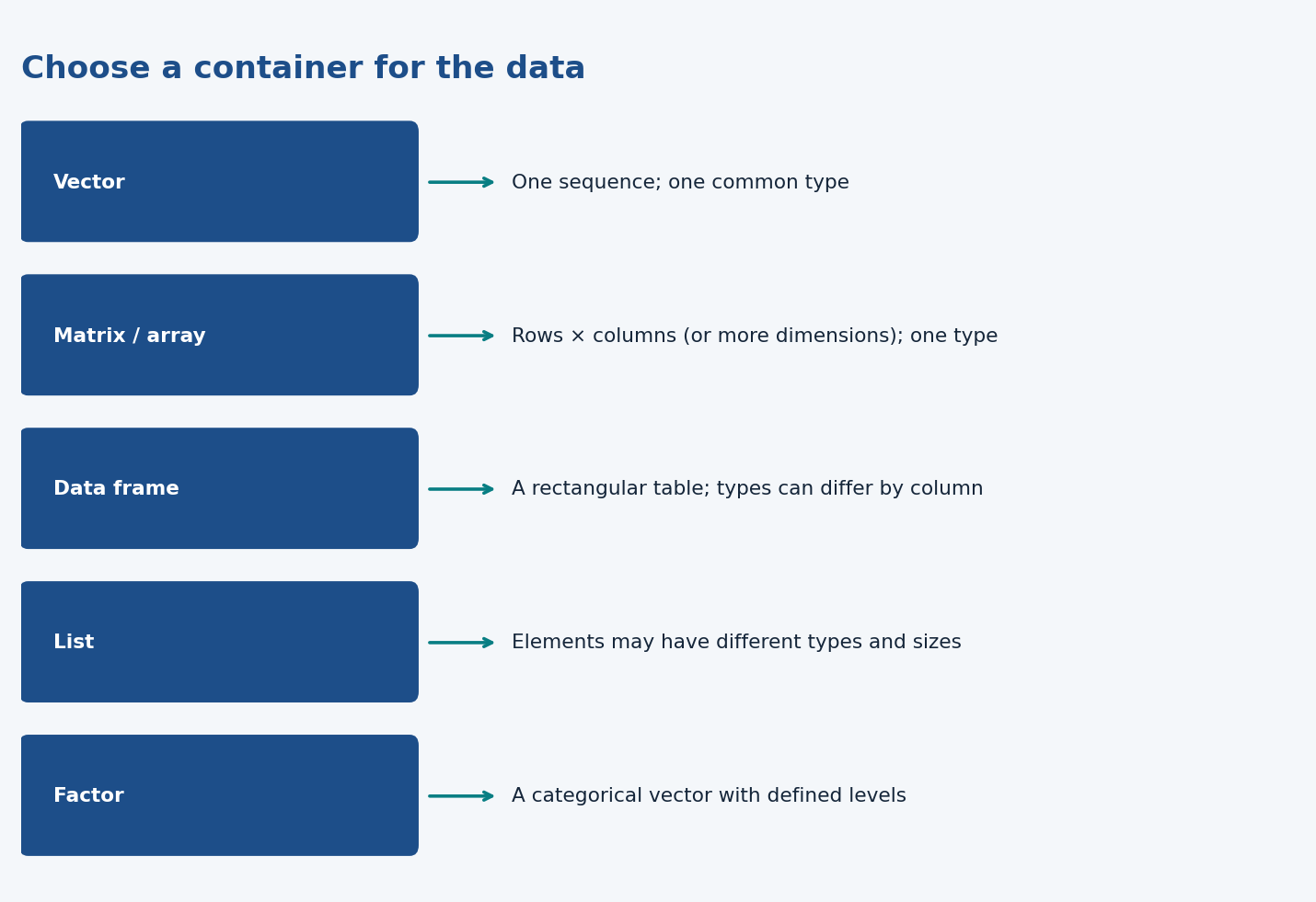
Containers. An atomic vector or matrix has one common type. A data frame can mix column types. A list can hold different kinds and sizes of objects. A factor stores categories.
Subsetting. x[2] takes an element; table[row, column] chooses a cell; table$height chooses a column. Logical conditions select matching observations.
Functions and missingness. mean, sum, median and round summarize/change values. na.rm = TRUE excludes missing entries from a summary; it does not recover them.
Conditions and loops. if/else selects one branch; for repeats instructions. Trace what each step does rather than memorizing code appearance.
Reusable work. Write functions for repeated calculations, check units, save scripts, and load installed packages using library().
What to be able to do
Be able to trace a short script, distinguish containers, explain missing-value handling and write a small function or condition. The example exams indicate question styles, not an exhaustive syllabus.
Got the big picture?Mark the overview done to fill this lecture's ring.
2Step 2 of 312–18 min
Detailed notes
Source:full presentation. Canvas lecture page checked 11 October 2026, 11:40 CEST. Existing lecture transcript used to clarify demonstrations; its older administrative dates are excluded. Examples labelled “illustration” are invented to explain the slide concepts.
Think of R as instructions applied to stored objects
An object is a named piece of data. A function is an instruction that takes inputs and returns a result. A script records these instructions so you can repeat the analysis.
Read this as “store these four numbers under the name height, then calculate their mean.” The console runs commands; a saved script makes the process reproducible. RStudio supplies editing, object inspection, help and plots around R.
Values, types and assignment
Type shown in the slides
Example
What it represents
Numeric, normally double
2.5, 2
Numbers, including decimal values
Integer
2L
Whole-number storage type
Character
"Amsterdam"
Text; quotes matter
Logical
TRUE, FALSE
A condition's truth value
Complex
3 + 2i
Numbers with real and imaginary parts
Raw
charToRaw("hello")
Bytes
Date/time objects
as.Date("2026-10-11")
Dates or timestamps represented using appropriate classes
NA means missing/unknown. It is not zero, the word “NA”, or false. It can be a missing value of different types. Date/time is a useful class of objects, rather than a separate primitive typeof() result.
Use <- to assign: age <- 24. The right-hand expression is evaluated and stored on the left. = can assign in many contexts, but <- keeps object assignment visually distinct from named function arguments such as na.rm = TRUE. Rightward assignment exists; the slides discourage it for readability.
R is case-sensitive: height and Height are different objects. Names cannot start with a digit and cannot contain arbitrary punctuation or spaces without special handling. Use simple meaningful names. ls() lists existing object names; typeof(x) checks a storage type; str(x) shows an object's structure. class(x) describes its class, which can convey more meaning than storage type.
mass <- 70
mass * 2       # 140
mass == 70     # TRUE: comparison, not assignment
Data structures: what container do you need?
Structure
Shape
Type rule
Example
Atomic vector
One-dimensional sequence
One common type
Several heights
Matrix
Rows and columns
One common type
Numerical test scores
Array
Multiple dimensions
One common type
Numerical measurements by person × test × day
Data frame
Rows and named columns
Columns can have different types; equal row counts
ID, name, height, injured
List
Collection of objects
Elements can have different types and sizes
A vector, table and model together
Factor
Categorical vector with levels
Stores category codes and category labels
Discipline or medal
NULL
Absence of an object/value
Not an ordinary missing observation
An empty result or absent list element
An atomic vector containing numbers and text is coerced to a common type, usually character. A list can preserve mixed element types. A data frame is list-like, but its columns must form a rectangular table.
R fills matrices by column unless you request byrow = TRUE. A matrix made with byrow = TRUE would instead have first row 168, 182. This difference matters when interpreting code.
A factor's labels are categories. Its internal integer codes are not quantities you should average. An ordered factor can explicitly encode an order where appropriate.
Subsetting: retrieve only the part you want
R indexing begins at 1. Square brackets select part of an object.
For a matrix or data frame, the comma separates rows, columns. An empty position means all rows or all columns. athletes["height"] returns a one-column data frame, whereas athletes$height normally returns the vector. For lists, x[1] preserves a sublist and x[[1]] extracts the element.
Logical filtering works because each TRUE selects its corresponding value. A missing comparison can yield NA, so missingness requires attention rather than assuming every comparison is true or false.
Functions and their arguments
A function call has the form function_name(arguments). Use ?mean or help("mean") for help, including argument names and defaults.
na.rm = TRUE tells these summaries to omit missing values. It does not restore the unobserved information or guarantee an unbiased estimate. Here it averages the three observed values.
names() attaches names to vector elements, not a new numerical value:
The slide calls this a “named function” in one place; the demonstration actually creates a named vector.
Rounding, floor and ceiling
Operation
Example
Meaning
round(x, 2)
round(3.146, 2) → 3.15
Nearest value to two decimal places
floor(x)
floor(3.8) → 3
Greatest integer no larger than x
ceiling(x)
ceiling(3.2) → 4
Smallest integer no smaller than x
Round to tens
round(47 / 10) * 10 → 50
Divide, round, multiply back
For negatives, floor(-3.2) is −4 and ceiling(-3.2) is −3. “Nearest 10th value” in the VO₂ exercise means rounding to multiples of ten, not necessarily one decimal place. In R, exact halfway cases use ties-to-even, so do not assume all halfway values round upward.
Relative VO₂ has units mL/kg/min. Multiplying by kg produces mL/min; dividing by 1,000 produces L/min. The slide example multiplies and divides by 1,000. State the output units. Functions can operate on whole vectors here, with corresponding elements multiplied. The last evaluated expression is returned; explicit return(...) also works.
Conditions: choose a branch
The comparison operators are <, >, <=, >=, ==, !=. Use == to compare equality; <- assigns. A scalar if condition must resolve to one nonmissing logical value.
Order matters. Test the highest threshold first. Once a branch is selected, subsequent branches are skipped. The second branch covers 175 up to but excluding 190, because the first branch already handled 190 and above. These are the exercise's illustrative labels, not universal physiological classifications.
Loops: repeat an instruction
for (h in height) {
  print(height_label(h))
}
Each iteration takes the next height, runs the same function, and prints its label. for (i in 1:4) iterates over indices instead. You can store results rather than only print them:
labels <- character(length(height))
for (i in seq_along(height)) {
  labels[i] <- height_label(height[i])
}
Vectorized functions often avoid an explicit loop, but knowing how to trace a loop helps you understand a script. Do not treat a code screenshot as something to memorize without following what changes at each step.
Libraries/packages
install.packages("ggplot2") downloads and installs a package; library(ggplot2) loads it for the current R session. Installation needs internet unless the files are already available. Once installed, packages work without downloading them again.
The slides show an ecosystem including plotting (ggplot2), wrangling (dplyr), dates (lubridate), reporting and interactive applications. You should recognize why packages exist rather than learn every logo. Lecture 4 develops wrangling and visualization.
What the ten slide exercises teach
Recognize data types.
Create vectors, a matrix and a data frame.
Name elements and print them.
Use mean, sum, median and round.
Handle missing values in summaries.
Round to a coarser increment.
Write a reusable VO₂ function.
Trace an if/else chain.
Repeat it for every group member.
Find relevant packages.
From the recording
Points the lecturer made in the lecture recording on Canvas that are not (fully) on the slides. Times refer to the recording.
03:52 — Reproducibility habits: start scripts with a header (goal, date, author, version) and comment the code; use RStudio projects to restore the workspace; record the R version because packages can break across versions. (not on slides)
10:59 — Integers (e.g. 5L) take less memory than numeric/double values, so calculations on large datasets are faster; the L suffix marks an integer. (Slides p. 10 (shows 2L, not the reason))
11:54 — Single and double quotes are equivalent for character strings in R; the rule is to be consistent. (not on slides)
13:20 — Assign with <-. The = sign also works but is discouraged because = is used to set function arguments (e.g. na.rm = TRUE); rightward assignment (->) is discouraged because readers expect the object name on the left. (Slides p. 11–12 (say 'discouraged'/'Don't do this' without the reason))
19:25 — Data retrieved from websites or APIs usually arrive as a list, which you have to unlist/convert; the data frame is the preferred structure for analysis in this course. (not on slides)
22:08 — In str() output, 'obs.' is the number of rows and 'variables' the number of columns, followed by each column's type; columns read from a CSV may come in as character and must be converted (e.g. as.numeric) before calculating. (Slides p. 23 (output shown, not explained))
36:10 — Name arguments explicitly (matrix(x, nrow = 2, ncol = 2)) so it is clear which value is which; named arguments may be given in any order. (not on slides)
37:17 — R indexing starts at 1, whereas Python starts at 0. (Slides p. 26 (R indexing only))
96:50 — source('file.R') loads functions saved in a separate script into your session, keeping the main script uncluttered. (not on slides)
Slide coverage map
Pages 1–6: motivation and environments; 7–16: values, assignment and inspection; 17–25: containers; 26–29: subsetting; 30–46: functions, naming, summaries, missingness, rounding and custom functions; 47–56: conditions and loops; 57–59: packages. Code screenshots were visually inspected; the explanations above provide readable equivalents.
Worked through the deep dive?Tick it off. Come back to any section whenever you need it.
3Step 3 of 35–8 min
Practice questions
Exactly two original practice questions. These use the concept/application style of the 2024 and 2022–2023 example exams, with new scenarios and values. Try each before opening its answer. The official example exams are on Canvas; save them for a later, exam-style session.
Question 1 — Trace a short script
Without running R, give the values of a, b, and answer. Explain the difference between a and b.
x <- c(12, NA, 18, 30)
a <- mean(x)
b <- mean(x, na.rm = TRUE)
answer <- x[c(1, 4)]
Show answer and rationale
a = NA; b = 20; answer = c(12, 30). The default mean cannot produce a known result with an unknown input. na.rm = TRUE averages the three observed values: (12 + 18 + 30)/3. Indexing begins at 1, so elements 1 and 4 are selected. Removing NA from a summary does not establish the missing value.
How did your answer compare?
Question 2 — Write a reusable function
Write an R function that takes a distance in kilometres and a duration in minutes, and returns average speed in km/h. What should it return for 6 km in 30 minutes? Assume positive duration.
12 km/h. Duration is converted to hours before division. Multiplying distance/duration by 60 is equivalent. The rationale is to preserve the requested units, not just obtain a plausible number.